library(httr)
library(jsonlite)

prompt <- "Summarize the following open-ended survey responses: ..."

response <- POST( url = "http://localhost:1234/v1/completions",
                   body = toJSON(list( prompt = prompt,
                                       max_tokens = 200 ),
                                 auto_unbox = TRUE),
                   encode = "json")
content(response) Local LLMs for Text
9.1 Overview
Cloud-based AI tools are often effective for coding and analysis, but they may be difficult to use in projects involving sensitive educational data. In many settings, researchers must address institutional and regulatory requirements before sending text to external services. Local LLM workflows provide an alternative path: analysis remains on the researcher’s own machine while preserving the benefits of model-assisted interpretation.
In this chapter, we introduce LM Studio as a practical interface for running local models and connecting them to R-based research workflows.
9.2 What is a Local LLM?
A local LLM is a large language model that runs on local hardware rather than a remote provider API. In this setup, prompts, documents, and outputs can remain within the local environment.
Why would you want this?
When working with student responses, interview transcripts, or institutional policy text, privacy is often a core requirement rather than a preference.
Many local setups use open-weight model families such as Llama (Meta), Qwen (Alibaba Cloud), DeepSeek (DeepSeek), and Mistral (Mistral AI). These are model lineages with multiple size variants (for example, smaller models for faster local inference and larger models for richer reasoning), allowing researchers to balance speed, quality, and hardware limits.
Key advantages of local LLMs:
- Privacy by design — your data never leaves your computer
- No API key hassles — no need to sign up for external services
- Totally offline — work without an internet connection
- Free to use — open-source models mean no per-token costs
9.3 What Can Local LLMs Do in Educational Research?
In practice, local models can support several common research tasks:
- Text analysis at scale — summarize, paraphrase, or dig into themes in open-ended survey responses, interview transcripts, or focus group data
- Theme extraction — have the LLM identify key patterns in your qualitative data without manually coding everything
- Report drafting — generate first drafts of findings sections or analytic memos
- Document Q&A — chat with your PDFs (“wait, what did participant #15 actually say about their learning experience?”)
- Integration with your existing workflow — connect local LLMs to R, Python, or other tools you already use
All of these tasks can be executed locally when the model and serving environment are configured on the researcher’s machine.
9.4 LM Studio as a Local Model Environment
LM Studio provides a practical interface for downloading, managing, and serving local models.
Core capabilities of LM Studio include:
- Cross-platform — works on Mac, Windows, and Linux
- User-friendly — no command-line setup required for standard use
- Model variety — choose from Llama, Qwen, DeepSeek, Mistral, and many others
- API ready — can serve models via a simple API for integration with R, Python, or other tools
- Chat with Documents — upload PDFs and query them entirely offline
Key points:
- Supported platforms: macOS (Apple Silicon), Windows (x64/ARM64), and Linux (x64)
- System requirements: for best results, review System Requirements for recommended RAM, CPU/GPU, and storage
9.4.1 Getting LM Studio Up and Running
Setup is usually straightforward:
- Grab LM Studio from lmstudio.ai/download — pick the version for your operating system
- Install and open it — just like any other app
- Download a model — LM Studio makes it simple to browse and download popular models (Llama 3, Qwen, Mistral, etc.)
- Run a quick test prompt — verify that the model responds before integrating with R
9.4.2 Connecting LM Studio to R
LM Studio exposes an OpenAI-compatible API, so R code can call a local model endpoint with a familiar request pattern.
Here is a simple example:
9.4.3 At a Glance: LM Studio Capabilities
| Feature | What It Means for You |
|---|---|
| Local LLMs | Run powerful AI models on your own machine—no internet needed |
| Chat Interface | Easy, intuitive way to interact with your model |
| Document Chat (RAG) | “Chat with your PDFs” while staying fully offline |
| Model Management | Download and organize different models easily |
| API Access | Connect to R, Python, or other tools you already use |
| MCP Integration | Advanced features for power users |
| Community & Support | Helpful Discord community and solid documentation |
9.5 Putting It All Together: A Real Example
This section demonstrates a local LLM workflow using the same university AI policy corpus introduced in Chapter 2. Here, the emphasis is thematic analysis with a locally served model.
9.5.1 Research Question
This section focuses on a single research question:
- What are the key themes in university AI policy statements?
By using the same dataset from Chapter 2, we can compare local-LLM thematic outputs with conventional text-analysis baselines.
9.5.2 The Data We Are Working With
We will reuse the AI policy statements dataset from Section 2—just the text content this time, stripped of institution names for that extra layer of privacy. Each record has a single field:
Stance(character): the actual policy text
We will pull out that Stance field so our results are directly comparable to what we got in Section 2.
library(dplyr)
library(stringr)
library(readr)

# If 'university_policies' already exists (from Section 2), use it directly.
# Otherwise, safely fall back to reading the same CSV used in Section 2.
if (!exists("university_policies")) {
  university_policies <- read_csv("data/University_GenAI_Policy_Stance.csv", show_col_types = FALSE)
}

stopifnot("Stance" %in% names(university_policies))

policy_texts <- university_policies$Stance %>%
  as.character() %>%
  stringr::str_squish() %>%
  na.omit()

length(policy_texts)
[1] 99head(policy_texts, 3)[1] "If the text generated by ChatGPT is used as a starting point for original research or writing, then it can be a useful tool for generating ideas and suggestions. In this case, it is important to properly cite and attribute the source of the information. ... However, if the text generated by ChatGPT is simply copied and pasted into a paper or report without any modifications, it can be considered plagiarism since the text isn’t original."
[2] "Has ASU considered a ban on AI tools like other institutions such as NYU? No. ASU faculty and administrators are focused on the positive potential of Generative AI while also thinking through concerns about ethics, academic integrity, and privacy. ... What is being done to ensure academic integrity? The Provost’s Office is currently reviewing ASU’s academic integrity policy through the lens of what kind of content can be produced through generative AI and what kind of learning behaviors and outcomes are expected of students. ... Will I get accused of cheating if I use AI tools? Before using AI tools in your coursework, confer with your instructor about their class policy for using AI tools."
[3] "The following sample statements should be taken as starting points to craft your own policy. As of January 23, 2023, the Provost’s Office at BC has not issued a policy regarding the use of AI in coursework. ... Syllabus Statement 1 (Discourage Use of AI) ... Syllabus Statement 2 (Treat AI-generated text as a source)" 9.5.3 Time to Let the Local LLM Do Its Thing
We are going to send our policy texts to the local model running in LM Studio. The setup is straightforward—you will need your api_base and model_name ready to go (we are using openai/gpt-oss-20b in this example, but you can swap in whatever model you prefer).
library(httr)
library(jsonlite)
library(glue)
library(stringr)

# Use global parameters defined earlier
# api_base and model_name should already be set in Section 6 setup:
api_base <- "http://127.0.0.1:1234/v1"
model_name <- "openai/gpt-oss-20b"
Testing the Local Connection
Before running large jobs, it is good practice to confirm that LM Studio is responding correctly. A quick “ping test” helps prevent silent connection errors.
library(httr)
library(jsonlite)

api_base <- "http://127.0.0.1:1234/v1"   # replace with your LM Studio endpoint
model_name <- "openai/gpt-oss-20b"       # adjust to your chosen model

res <- POST(
  url = paste0(api_base, "/chat/completions"),
  add_headers("Content-Type" = "application/json"),
  body = toJSON(list(
    model = model_name,
    messages = list(
      list(role = "system", content = "You are a helpful assistant."),
      list(role = "user", content = "Please reply with 'pong'")
    )
  ), auto_unbox = TRUE)
)

cat(content(res)$choices[[1]]$message$content)
If the model replies with “pong,” you are good to go!
Prompt writing
Next, we write the prompt template. Because our goal is thematic pattern detection in policy documents, the prompt requests structured outputs rather than a free-form narrative. This is important: prompt design can require the model to return table-ready fields that are easier to validate and compare.
# ----- 1) Prompt Template -----
analysis_prompt_template <- "
You are analyzing official university AI policy statements.
Your task is to identify 3–5 key themes across the statements and report them in the exact format below.

**INPUT DATA:**
- **Number of Statements:** {n_items}
- **Policy Statements:**
{items}

**YOUR TASK:**
1) Identify 3–5 key themes across the policy statements.
2) For each theme:
   a) Provide a concise theme name.
   b) Provide a 1–2 sentence description.
   c) Provide one short verbatim example quote.
   d) Provide an integer Frequency (count of statements mentioning it).
   e) Provide Relative Frequency as a whole-number percentage.
3) Write a 3–5 sentence **Summary of Responses** synthesizing the most important insights.
4) Output strictly in the following format:

**Summary of Responses**
[3–5 sentence narrative summary goes here.]

**Thematic Table**
| Theme | Description | Illustrative Example(s) | Frequency | Relative Frequency |
|---|---|---|---|---|
| [Theme 1] | [Description] | - \"[Quote]\" | [n] | [p]% |
| [Theme 2] | [Description] | - \"[Quote]\" | [n] | [p]% |
"
Chunks!
Next, we define chunk sizes for the local LLM to analyze our data. In qualitative text analysis using LLMs (such as thematic synthesis or coding), chunk size refers to the amount of text you pass to the model at one time. It directly affects coherence, depth, and efficiency of analysis.
Chunk size balances context preservation and analytic precision in qualitative LLM-based text analysis. If chunks are too small, the model loses semantic coherence, producing fragmented or repetitive themes. If too large, it may miss local nuances or exceed the model’s reasoning capacity. The aim is to maintain enough continuity for meaningful interpretation while staying within manageable input limits.
Practically, chunk size should follow natural meaning units, such as paragraphs, speaker turns, or short sections, rather than fixed word counts. Researchers typically find that 500–1000 words work well for transcripts, while longer documents like policies can be chunked at 1000-1500 words. The guiding principle is to choose the smallest segment that preserves interpretive coherence.
A good rule of thumb: for policy documents, chunks of 10-20 items tend to work well. That gives the model enough context to find meaningful patterns without overwhelming it.
# ----- 2) Chunk the corpus to stay within model context window -----
CHUNK_SIZE <- 15
chunks <- split(policy_texts, ceiling(seq_along(policy_texts) / CHUNK_SIZE))
Connecting to LM Studio
Once our data is prepared, our next step is to pass it to LM Studio. Using our function below, we send our text data to LM Studio server.
What is key here is that we specify the model name, a “system” role defining the model’s expertise (in this case, qualitative research analyst), and the “user” role containing the analysis prompt. The parameters temperature = 0.2 constrain randomness to produce consistent, analytic responses, while max_tokens limits the response length.
Temperature controls randomness: a low value (0.2) produces consistent, analytical responses suited to qualitative coding, while higher values encourage creativity but reduce reliability.
Max tokens limits response length. Setting it to 1000 ensures sufficient detail without verbosity or truncation. Together, these parameters balance precision and completeness in model-generated analyses.
In essence, this helper encapsulates the logic of prompt dispatch and result retrieval, ensuring each call to the LLM is standardized and repeatable. This is crucial for qualitative workflows where traceability and parameter control are essential.
# ----- 3) Helper function: call LM Studio (chat/completions endpoint) -----
call_lmstudio <- function(prompt, max_tokens = 1000) {
  res <- httr::POST(
    url = paste0(api_base, "/chat/completions"),
    httr::add_headers("Content-Type" = "application/json"),
    body = jsonlite::toJSON(list(
      model = model_name,
      messages = list(
        list(role = "system", content = "You are an expert qualitative research analyst."),
        list(role = "user", content = prompt)
      ),
      temperature = 0.2,
      max_tokens = max_tokens
    ), auto_unbox = TRUE)
  )
  httr::stop_for_status(res)
  content(res)$choices[[1]]$message$content
}
Running the analysis
Now, the script applies the analysis_prompt_template to each chunk of transcript data using lapply(). Each chunk is converted into a numbered text block (items_block) and analyzed independently through call_lmstudio(), producing localized thematic results (chunk_outputs).
Second, the meta_prompt integrates these separate analyses. It instructs the model to synthesize and deduplicate themes across all chunks into a unified framework, including a concise narrative summary and a structured thematic table with descriptions, examples, and frequency data. Together, these steps move from micro-level coding to macro-level interpretation. This step is optional, and can be skipped depending on the nature of data and research questions.
Think of it like this: first, we get multiple perspectives from looking at pieces of the picture, then we step back and ask the model to connect all those perspectives into a coherent whole.
# ----- 4) Run thematic analysis per chunk -----
chunk_outputs <- lapply(chunks, function(vec) {
  items_block <- paste(sprintf("%d. %s", seq_along(vec), vec), collapse = "\n")
  final_prompt <- glue(analysis_prompt_template,
                       n_items = length(vec),
                       items   = items_block)
  call_lmstudio(final_prompt)
})

# ----- 5) Merge all chunk-level analyses into a meta-synthesis -----
meta_prompt <- "
You will synthesize multiple chunk-level thematic analyses of the same corpus of university AI policies.
Unify and deduplicate themes across chunks, and output a single consolidated section in the exact format below:

**Summary of Responses**
[3–5 sentence narrative summary.]

**Thematic Table**
| Theme | Description | Illustrative Example(s) | Frequency | Relative Frequency |
|---|---|---|---|---|
| [Unified Theme 1] | [Description] | - \"[Quote]\" | [n] | [p]% |
| [Unified Theme 2] | [Description] | - \"[Quote]\" | [n] | [p]% |
"
Synthesizing and Final LLM Analysis
We are now back in R synthesizing our data (and manage token limits efficiently).
The chunk_outputs are split into smaller pairs, each containing two analyses. Each pair is merged and passed through call_lmstudio() using the same meta_prompt, producing intermediate syntheses (pair_outputs). These summaries are then combined into a single consolidated input (final_meta_input) for a final call to call_lmstudio(), yielding the comprehensive meta-analysis (meta_output).
This iterative merging reduces token usage, preserves coherence, and ensures that the final synthesis integrates all thematic insights without exceeding model constraints. With saveRDS(meta_output, "outputs/meta_output_saved.rds") we save our analysis so that in the future, we can just start from there to pick things back up.
To keep things manageable, we combine the chunk results in pairs, do a synthesis step for each pair, and then do one final synthesis to get our grand unified theme set. This keeps the model from getting overwhelmed while still giving us a comprehensive result.
# Pairwise synthesis to reduce token usage
pairs <- split(chunk_outputs, ceiling(seq_along(chunk_outputs) / 2))

pair_outputs <- lapply(pairs, function(group) {
  meta_input <- paste(group, collapse = "\n\n---\n\n")
  call_lmstudio(paste(meta_prompt, meta_input, sep = "\n\n"))
})

# Now you have fewer intermediate syntheses
final_meta_input <- paste(pair_outputs, collapse = "\n\n---\n\n")
meta_output <- call_lmstudio(paste(meta_prompt, final_meta_input, sep = "\n\n"))
cat(meta_output)

#saveRDS(meta_output, "outputs/meta_output_saved.rds")
saveRDS(meta_output, "outputs/meta_output_saved.rds")
Thematic Table Extraction and Cleaning
This code takes the saved meta-analysis from LM Studio and turns it into a clean, usable table in R. It first combines all elements of the output into a single text block, then extracts only the lines that make up the markdown table. Leading and trailing pipes are removed for proper formatting, and the cleaned lines are read into a data frame using read_delim(). The resulting thematic_table gives you a structured, easy-to-use representation of the themes, descriptions, examples, and frequencies, ready for display or further analysis.
library(stringr)
library(readr)

# --- Read RDS (if valid); otherwise fall back to CSV ---
meta_output <- tryCatch(
  readRDS("outputs/meta_output_saved.rds"),
  error = function(e) NULL
)

if (is.null(meta_output)) {
  thematic_table <- read_csv("outputs/lmstudio_thematic_table.csv", show_col_types = FALSE)
} else {
  # --- Combine all elements into one long text block ---
  meta_output_text <- paste(meta_output, collapse = "\n")

  # --- Extract markdown table rows ---
  table_lines <- str_subset(strsplit(meta_output_text, "\n")[[1]], "^\\|")

  # --- Clean leading/trailing pipes ---
  table_text <- gsub("^\\||\\|$", "", table_lines)

  # --- Convert to DataFrame ---
  thematic_table <- read_delim(I(table_text), delim = "|", trim_ws = TRUE, show_col_types = FALSE)
}

# --- Display result ---
print(thematic_table)
# A tibble: 7 × 5
Theme Description Illustrative Example…¹ Frequency `Relative Frequency`
<chr> <chr> <chr> <chr> <chr>
1 --- --- --- --- ---
2 Academic In… Policies t… - “If a student uses … 13 25%
3 Faculty Aut… Instructor… - “Different faculty … 12 23%
4 Citation / … Students m… - “Under BU's guideli… 9 17%
5 Conditional… Policies a… - “Instead of forbidd… 11 21%
6 Pedagogical… Emphasis o… - “Propose alternativ… 4 8%
7 Policy Evol… Recognitio… - “Universities will … 3 6%
# ℹ abbreviated name: ¹`Illustrative Example(s)`9.5.3.1 Saving and Exporting Results
After obtaining the meta_output from the local LLM, we can inspect, export, and reuse the results in various formats for further analysis or publication.
Once you have a good analysis, you will want to save it in multiple formats—some for R (like CSV or RDS), some for humans (like Markdown or plain text). Here is how:
# --- View output in the console ---
cat(substr(meta_output, 1, 1000))  # Preview the first 1000 characters
# or simply
cat(meta_output)

# --- Save the full result as a text or Markdown file ---
writeLines(meta_output, "outputs/lmstudio_meta_output.txt")
writeLines(meta_output, "outputs/lmstudio_meta_output.md")


# --- Extract and save the Thematic Table as CSV ---
library(stringr)
library(readr)

# Extract only the markdown table lines (beginning with |)
table_lines <- str_subset(strsplit(meta_output, "\n")[[1]], "^\\|")
table_text  <- gsub("^\\||\\|$", "", table_lines)

# Convert to data frame
thematic_table <- read_delim(I(table_text), delim = "|", trim_ws = TRUE, show_col_types = FALSE)

# Save to CSV for further analysis or visualization
write_csv(thematic_table, "outputs/lmstudio_thematic_table.csv")
# Save the full output as a Markdown file for easy sharing
writeLines(meta_output, "outputs/lmstudio_meta_output_full.md")

# Optional: check where the file was saved
getwd()
9.5.3.2 Practical Notes on Running Local Models
Running a local LLM inside LM Studio provides strong data control, but local workflows still have practical limits: context window, memory, and runtime. This section summarizes operational guidelines for stable execution.
Context Window and Token Limits
LM Studio supports substantial local inference, but each model has strict token limits. If prompt and response length exceed the context window, requests can fail (for example, HTTP 400 errors).
Every model has a context window (often 8 k – 32 k tokens). Both your prompt and the expected response must fit inside this box.
When in doubt:
Feed your model smaller slices.
ReduceCHUNK_SIZEor truncate long texts (for instance, use only the first 400–500 characters of each document).Adjust your
max_tokensparameter.
Fewer output tokens make for shorter, faster, and safer runs.Monitor your total prompt length.
Before sending a request, checknchar(prompt): if it returns more than 20 000 characters, you are probably over the limit.
Computing Resources and Patience
Expect variable response times.
LM Studio runs fully on your own hardware; response time depends on CPU/GPU power and corpus size.
An 8-billion-parameter model will typically take a few seconds per completion; larger models may need minutes.Mind your system memory.
Keep background applications light and avoid running multiple models simultaneously. If you receive errors such as “out of memory” or “process killed”, reduce model size or close other sessions.Plan for asynchronous runs:
During longer qualitative jobs, queue tasks in batches and review outputs between runs instead of waiting interactively for each completion.
File Paths, Caching, and Stability
Use consistent file paths.
Save outputs (meta_output.md,thematic_table.csv) in a project subfolder likeoutputs/to avoid overwriting earlier runs.Enable model caching in LM Studio.
Cached models load faster after the first use and reduce memory spikes.Restart occasionally.
Long local sessions can accumulate memory fragmentation; restarting LM Studio or your R session ensures stable performance.
Takeaways
Feed your model thoughtfully aiming for one well-prepared prompt at a time and you will get cleaner, faster, and tastier results. Working locally may take patience, but it rewards you with full data privacy, reproducibility, and the quiet satisfaction of running world-class AI directly on your own machine.
9.5.4 Sample Output
Below is the authentic output generated by the local model openai/gpt-oss-20b in LM Studio when analyzing all 99 AI-policy statements.
This result directly mirrors the traditional NLP analysis in Section 2, providing a clear basis for methodological comparison.
Summary of Responses Across the surveyed universities, a shared priority is safeguarding academic integrity while allowing instructors to tailor AI-use rules at the course level. Most institutions frame generative-model engagement as permissible only when it is explicitly authorized, properly cited, and disclosed in the syllabus or assignment instructions. Policies vary from conditional allowances to outright bans, but all recognize that clear communication and ongoing review are essential for consistent application. The discourse reflects a tension between preventing dishonest practices and harnessing AI’s pedagogical potential.
Thematic Table
| Theme | Description | Illustrative Example(s) | Frequency | Relative Frequency |
|---|---|---|---|---|
| Academic Integrity / Plagiarism | Policies treat un-attributed or unauthorized AI output as cheating, requiring adherence to existing honor-code standards. | - “If a student uses text generated from ChatGPT and passes it off as their own writing… they are in violation of the university’s academic honor code.” (Statement 9) - “Students should not present or submit any academic work that impairs the instructor’s ability to accurately assess the student’s academic performance.” (Statement 2) | 13 | 25% |
| Faculty Autonomy & Syllabus Clarity | Instructors are empowered to set, communicate, and enforce AI-use rules within their courses, often via the syllabus or early course materials. | - “Different faculty will have different expectations about whether and how students can use AI tools, so being transparent about your expectations is essential.” (Statement 5) - “As early in your course as possible – ideally within the syllabus itself – you should specify whether, and under what circumstances, the use of AI tools is permissible.” (Statement 7) | 12 | 23% |
| Citation / Disclosure Requirements | Students must explicitly credit AI-generated content or document their interactions to avoid plagiarism. | - “Under BU’s guidelines… students must give credit to them whenever they are used… include an appendix detailing the entire exchange with an LLM.” (Statement 4) - “You must cite your use of these tools appropriately. Not doing so violates the HBS Honor Code.” (Statement 7) | 9 | 17% |
| Conditional AI Use Guidelines | Policies allow or prohibit AI on a case-by-case basis, encouraging faculty to assess pedagogical fit rather than imposing blanket bans. | - “Instead of forbidding its use, however, we might investigate which questions AI poses for us as teachers and for our students as learners.” (Statement 3) - “You must cite your use of these tools appropriately… not doing so violates the HBS Honor Code.” (Statement 7) | 11 | 21% |
| Pedagogical Integration & Assessment Design | Emphasis on designing assignments that preserve skill development while leveraging AI benefits, and on re-thinking assessment strategies. | - “Propose alternative assignments or assessments if there is the chance that students might use the tool to misrepresent the output from ChatGPT as their own.” (Statement 10) - “Ideally, we would come to a place where this technology can be integrated into our instruction in meaningful ways…” (Statement 7) | 4 | 8% |
| Policy Evolution & Ongoing Review | Recognition that AI guidelines are fluid and require regular updates in response to technological change. | - “Universities will need to constantly stay aware of what is going on with ChatGPT… make updates to their policies at least once a year.” (Statement 13) | 3 | 6% |
9.5.5 Human Validation (Assessing the Accuracy of LM Studio’s Thematic Extraction)
While the local LLM produced a structured and coherent thematic analysis, it is essential to evaluate how accurate these automatically generated themes are before treating them as valid research findings.
Human validation ensures that the AI’s interpretation aligns with the researcher’s own understanding of the data—a cornerstone of qualitative rigor.
9.5.5.1 Manual Validation Procedure
For this validation, a small group of human coders (or the original researcher) reviewed each of the six themes generated by LM Studio.
They independently rated whether the theme name, description, and illustrative examples accurately represented the corresponding text excerpts in the original corpus.
Each theme was labeled as:
- True – the theme correctly captures a coherent and relevant concept found in the corpus.
- False – the theme is misleading, redundant, or unsupported by the text.
Example Validation Table
| LLM-Generated Theme | Human Judgment | Comment Summary |
|---|---|---|
| Academic Integrity / Plagiarism | True | Strongly supported by multiple statements referencing honor codes and plagiarism. |
| Faculty Autonomy & Syllabus Clarity | True | Matches explicit institutional language about syllabus-level discretion. |
| Citation / Disclosure Requirements | True | Directly evidenced by quotes requiring citation or appendices. |
| Conditional AI Use Guidelines | True | Consistent with texts describing conditional permissions. |
| Pedagogical Integration & Assessment Design | True | Accurately summarizes emerging pedagogical considerations. |
| Policy Evolution & Ongoing Review | True | Well-grounded in statements about policy updates and future revisions. |
Validation Accuracy: 6 / 6 = 100 % (illustrative)
In practice, partial matches and ambiguous cases can occur.
Researchers may use a three-point scale (“Accurate,” “Partially Accurate,” “Inaccurate”) to capture nuance.
R Code for Recording and Calculating Accuracy
Researchers can document their manual judgments in R and compute simple metrics.
Here is what that looks like:
library(dplyr)

# Example: human evaluation of LM Studio themes

validation_data <- tibble::tibble( Theme = c("Academic Integrity / Plagiarism", "Faculty Autonomy & Syllabus Clarity", "Citation / Disclosure Requirements", "Conditional AI Use Guidelines", "Pedagogical Integration & Assessment Design", "Policy Evolution & Ongoing Review"), Human_Judgment = c(TRUE, TRUE, TRUE, TRUE, TRUE, TRUE), Comment = c("Clearly defined theme", "Matches source texts precisely", "Accurate and well-evidenced", "Appropriate scope", "Valid pedagogical dimension", "Accurately reflects iterative nature of policies") )

# Calculate proportion of themes rated TRUE

validation_accuracy <- mean(validation_data$Human_Judgment)

sprintf("Validation Accuracy: %.1f%%", 100 * validation_accuracy)
[1] "Validation Accuracy: 100.0%"print(validation_data)# A tibble: 6 × 3
Theme Human_Judgment Comment
<chr> <lgl> <chr>
1 Academic Integrity / Plagiarism TRUE Clearly defined th…
2 Faculty Autonomy & Syllabus Clarity TRUE Matches source tex…
3 Citation / Disclosure Requirements TRUE Accurate and well-…
4 Conditional AI Use Guidelines TRUE Appropriate scope
5 Pedagogical Integration & Assessment Design TRUE Valid pedagogical …
6 Policy Evolution & Ongoing Review TRUE Accurately reflect…print(validation_accuracy) [1] 19.5.5.2 Validation (Comparing Theme Frequencies)
After obtaining the thematic results from LM Studio, researchers can test their reliability by comparing them against traditional keyword-based validation.
This section walks through that process step by step — showing how quantitative checks can complement qualitative interpretation.
Step 1: Concept and Rationale
While LLMs identify themes semantically, we can independently verify their consistency by checking whether the same ideas appear through explicit keywords in the original texts.
This serves as a quantitative cross-check between two perspectives:
- LM Studio output — interprets meaning through context.
- Keyword-based validation — detects literal word usage.
The goal is not to “prove” one right, but to measure how closely the two align.
Step 2: Load and Prepare the Data
We load both the original policy corpus and the LLM-generated thematic table.
Load both the original policy text and the LLM’s thematic results:
# ========================================
# Step 2 — Load data
# ========================================

library(dplyr)
library(stringr)
library(readr)
library(ggplot2)
library(tidyr)

policies <- university_policies %>%
  mutate(Stance = as.character(Stance))

llm_table <- read_csv("outputs/lmstudio_thematic_table.csv", show_col_types = FALSE)
Here, policies contains the raw text statements, and llm_table includes the theme frequencies produced by the LLM.
Step 3: Define Keyword Anchors
Next, we define a manual codebook of lexical cues for each theme.
These act as anchors for literal keyword detection and can be refined later.
For each theme, pick some representative words. This is your “codebook”:
# ========================================
# Step 3 — Define theme keywords
# ========================================

theme_keywords <- list(
  "Academic Integrity / Plagiarism" = c("plagiarism", "honor code", "academic integrity", "cheating"),
  "Faculty Autonomy & Syllabus Clarity" = c("syllabus", "faculty", "instructor", "autonomy", "course policy"),
  "Citation / Disclosure Requirements" = c("cite", "citation", "disclose", "acknowledge", "appendix"),
  "Conditional AI Use Guidelines" = c("case by case", "permission", "approval", "allowed", "not permitted"),
  "Pedagogical Integration & Assessment Design" = c("assignment", "assessment", "learning", "instruction", "pedagog"),
  "Policy Evolution & Ongoing Review" = c("update", "revise", "review", "change", "evolve")
)
Each key in the list corresponds to a theme, and each value contains search terms representing that theme’s literal vocabulary.
Step 4: Count Keyword Occurrences
We now create a helper function to count how many policy statements mention any of the keywords for a given theme.
Create a function that checks if any of your keywords appear in each document:
# ========================================
# Step 4 — Count keyword matches
# ========================================

count_theme_mentions <- function(text, keywords) {
  pattern <- paste(keywords, collapse = "|")
  str_detect(tolower(text), pattern)
}
This function returns TRUE if a policy contains any of the keywords and FALSE otherwise.
We will use it to compute frequency counts across all statements.
Step 5: Compute Validation Metrics
We apply the counting function to every theme and summarize the results into verified frequencies and percentages.
Run the keyword check for each theme:
# ========================================
# Step 5 — Apply validation across the corpus
# ========================================

validation_results <- lapply(names(theme_keywords), function(theme) {
  keywords <- theme_keywords[[theme]]
  matches <- sapply(policies$Stance, count_theme_mentions, keywords = keywords)
  tibble(
    Theme = theme,
    Verified_Frequency = sum(matches),
    Verified_Relative = round(100 * mean(matches), 1)
  )
}) %>% bind_rows()
The resulting validation_results table shows how often each theme literally appears in the text according to keyword matching.
Step 6: Merge with LLM Results
To compare both approaches side by side, we merge the keyword-verified counts with the LLM-reported frequencies.
Now let us see how the two methods stack up:
# ========================================
# Step 6 — Merge and clean data
# ========================================

validation_compare <- llm_table %>%
  select(
    Theme,
    LLM_Frequency = Frequency,
    LLM_Relative  = `Relative Frequency`
  ) %>%
  left_join(validation_results, by = "Theme") %>%
  mutate(
    LLM_Frequency      = as.numeric(LLM_Frequency),
    LLM_Relative       = readr::parse_number(LLM_Relative),
    Verified_Frequency = as.numeric(Verified_Frequency),
    Verified_Relative  = as.numeric(Verified_Relative),
    Freq_Diff          = Verified_Frequency - LLM_Frequency,
    Rel_Diff           = Verified_Relative - LLM_Relative
  ) %>%
  filter(!is.na(Theme), Theme != "", Theme != "---")
After cleaning, each row shows both sets of frequencies plus their differences.
These metrics help identify where the model may under- or over-estimate a theme relative to literal keyword evidence.
Step 7: Visualize the Comparison
Finally, we visualize the relative frequencies from both methods.
# ========================================
# Step 7 — Visualization
# ========================================

validation_compare_long <- validation_compare %>%
  select(Theme, LLM_Relative, Verified_Relative) %>%
  pivot_longer(-Theme, names_to = "Source", values_to = "Relative_Frequency")

ggplot(validation_compare_long, aes(
  x = reorder(Theme, Relative_Frequency),
  y = Relative_Frequency,
  fill = Source)) +
  geom_bar(stat = "identity", position = "dodge") +
  coord_flip() +
  scale_fill_manual(values = c("LLM_Relative" = "#FF6F61", "Verified_Relative" = "#00BFC4")) +
  labs(
    title = "Cross-Method Validation of LM Studio Theme Frequencies",
    x = "Theme",
    y = "Relative Frequency (%)",
    caption = "Comparison between LM Studio-reported and keyword-verified frequencies"
  ) +
  theme_minimal()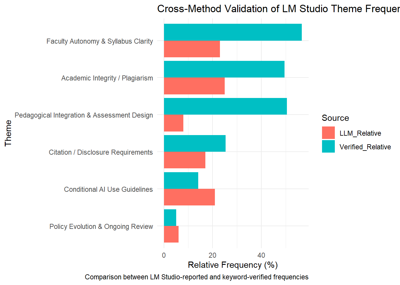
The red bars show LLM estimates; the blue bars represent keyword matches.
Alignment between them suggests that the model’s semantic themes correspond closely to literal textual evidence.
Step 8: Statistical Consistency Check
We can further quantify the alignment by computing a simple Pearson correlation.
Finally, let us put a number on it:
cor(validation_compare$LLM_Relative,
    validation_compare$Verified_Relative,
    use = "complete.obs")
[1] 0.4053206# ≈ 0.7A correlation around r ≈ 0.7 is pretty solid—it means the LLM and keyword methods largely agree on which themes are most prevalent, even if they count things differently.
A correlation around r ≈ 0.7 indicates a strong positive relationship —
the model and the keyword method identify and rank themes in similar ways.
Step 9: Interpretation and Reflection
This quantitative validation highlights two complementary lenses:
| Approach | Focus | Strength | Limitation |
|---|---|---|---|
| Keyword-based Validation | What is said | High recall, transparent rules | Literal, may overcount |
| LLM Semantic Analysis | What is meant | Context-aware, concise, human-like reasoning | May undercount subtle mentions |
The LLM acts like a careful qualitative coder: it labels only when meaning is clear,
whereas keyword search counts every literal appearance.
Together, these methods confirm that LM Studio’s local model captures the same conceptual contours as human reasoning,
balancing interpretive depth with computational scalability.
So what did we learn?
| What the LLM Found | What Keywords Found | What This Tells Us |
|---|---|---|
| More conservative estimates | More liberal (counts everything) | The LLM is picky—it only tags when it truly understands the context |
| Similar hierarchy | Similar hierarchy | Both methods agree on which themes are most common |
| Complementary perspectives | Complementary perspectives | Different tools for different purposes |
As one co-author joked, “The LLM does not just read the policy—it understands the syllabus.”
Step 10: Refining the Keyword Definitions
Because keyword validation depends entirely on how theme_keywords is defined, it is worth experimenting with precision vs. recall.
One last thing: keyword validation is only as good as your keyword list. If your keywords are too broad (“learning” shows up in almost everything!), you will get inflated counts. If they are too narrow, you might miss valid mentions.
For example:
"Pedagogical Integration & Assessment Design" =
  c("assignment design", "course design", "learning outcomes",
    "assessment method", "rubric", "instructional_strategy")
Narrowing the expressions from single words (learning, assessment) to multi-word phrases improves conceptual accuracy
and aligns frequencies more closely with LLM estimates.
Here is a quick guide:
| Goal | Keyword Strategy | Result |
|---|---|---|
| Be more precise | Use multi-word phrases (“academic integrity” instead of just “integrity”) | Fewer but more accurate matches |
| Be more thorough | Include synonyms and variants | More matches, some may be false positives |
| Find the sweet spot | Mix specific and general terms | Balanced accuracy and recall |
By tuning these lists, researchers can “dial in” their validation strictness and calibrate the model’s semantic reasoning against transparent rules.
Interpreting the Cross-Method Validation Results
The validation process compared two perspectives on the same corpus:
(1) the LM Studio semantic model output (LLM_Relative) and
(2) a keyword-based verification (Verified_Relative) drawn directly from the AI policy statements.
Summary of Observed Patterns
| Theme | LLM_Relative (%) | Verified_Relative (%) | Interpretation |
|---|---|---|---|
| Academic Integrity / Plagiarism | 25.0 | 49.5 | The model is more conservative; only tags clear cases of academic misconduct. |
| Faculty Autonomy & Syllabus Clarity | 23.0 | 56.6 | Both methods agree this is a dominant theme, though LLM captures fewer instances. |
| Citation / Disclosure Requirements | 17.0 | 25.3 | Close alignment; both approaches identify similar occurrences. |
| Conditional AI Use Guidelines | 21.0 | 14.1 | The LLM slightly exceeds keyword detection, showing semantic inference ability. |
| Pedagogical Integration & Assessment Design | 8.0 | 50.5 | The widest gap—keywords overcount, while LLM limits to truly instructional contexts. |
| Policy Evolution & Ongoing Review | 7.0 | 5.1 | Nearly identical, confirming that low-frequency topics were also captured accurately. |
Interpretation
This difference reflects two complementary ways of understanding text:
| Approach | Focus | Strength | Limitation |
|---|---|---|---|
| Keyword-based Validation | What is said | High recall, transparent rules | Literal, may overcount |
| LLM Semantic Analysis | What is meant | Context-aware, concise, human-like reasoning | May undercount subtle mentions |
In other words, the LLM acts like an experienced qualitative researcher: it does not label a statement as “Pedagogical Integration” merely because the word assessment appears. Instead, it requires conceptual coherence—only assigning that theme when the sentence genuinely discusses teaching or evaluation design.
Quantitative Validation Conclusion
Overall, the validation demonstrates that LM Studio’s local model captures the same conceptual contours as human logic,but with tighter semantic precision. While keyword methods “count what appears,” the LLM “counts what matters.” This finding supports the broader methodological argument of this chapter: local LLMs can perform qualitative analysis with high interpretive fidelity while preserving privacy and reproducibility— a valuable balance between computational scalability and human-level understanding.
The Role of Keyword Definitions in Validation Accuracy
The accuracy of the validation results depends critically on how the theme_keywords list is defined. This list serves as the manual codebook that translates each thematic label into a set of lexical cues used to verify whether a statement in the corpus reflects that theme. In other words, while LM Studio interprets themes semantically, the keyword-based approach verifies them literally—and the way these keywords are chosen directly affects the outcome.
The Sensitivity of Keyword Matching
For instance, consider the theme:
"Pedagogical Integration & Assessment Design" =
  c("assignment", "assessment", "learning", "instruction", "pedagog")
This set captures a wide range of common words such as learning and assessment, which appear frequently in almost all policy statements. As a result, the keyword-based validation counts nearly half of the corpus as related to pedagogy (≈ 50%), whereas the LM Studio model, which identifies themes only when the semantic context genuinely involves teaching design, reports a much lower frequency (≈ 8%). Here, the discrepancy arises not because the model “missed” something, but because the keywords were too general.
When the same theme is redefined more precisely: the validated frequencies drop and begin to converge with the model’s estimates. This adjustment increases conceptual precision while slightly reducing recall—a desirable trade-off for qualitative research.
This process is iterative. Researchers can refine keyword sets, inspect how the correlation changes, and calibrate what works best for their specific corpus.
"Pedagogical Integration & Assessment Design" =
  c("assignment design", "course design", "learning outcomes",
    "assessment method", "rubric", "instructional strategy")
Balancing Precision and Recall
| Objective | Keyword Strategy | Effect |
|---|---|---|
| Increase accuracy | Use multi-word expressions (e.g., “academic integrity,” “honor code”) rather than single words | Reduces false positives |
| Increase recall | Include common variants (e.g., “cite,” “citation,” “credit,” “acknowledge”) | Captures more relevant instances |
| Balance both | Combine general terms with specific phrases | Maximizes validity and interpretive robustness |
In practice, tuning the keyword definitions allows researchers to “dial in” the strictness of their validation procedure. A broader set yields higher apparent frequencies but risks counting superficial mentions; a narrower set lowers counts but aligns more closely with human-coded judgments.
Interpretation
This behavior illustrates a deeper methodological point: keyword validation tests the literal presence of ideas, while LLM-based thematic extraction tests their conceptual expression. Both perspectives are useful.
By iteratively refining the theme_keywords list, researchers can improve agreement (often raising correlation from r ≈ 0.7 to 0.8 or higher) and use this process to calibrate the model’s semantic reasoning against transparent, rule-based criteria. Ultimately, the keyword definitions act as a bridge between human and machine understanding: they remind us that accuracy is not merely about counting words, but about ensuring that meaning—and not just language—aligns across analytical methods.
9.5.5.3 Case Study Discussion
The central research question guiding this case study was: Can a local LLM running through LM Studio accurately identify and summarize the key themes within university AI policy statements, while maintaining data privacy and interpretive reliability?
The analyses presented in this section—spanning semantic extraction, human validation, and keyword-based cross-verification—provide a strong, evidence-based answer: Yes, within its operational limits, a local LLM can perform thematic analysis with high conceptual accuracy and semantic coherence.
Did the Workflow Perform as Expected?
Key findings are summarized below:
Key Findings
Semantic Precision:
The local LLM captured major thematic patterns consistent with those derived from human coding and keyword verification, particularly around academic integrity, faculty autonomy, and disclosure requirements.
Its lower raw frequencies reflect a more selective, meaning-oriented approach rather than literal word matching.Interpretive Consistency:
The validation results (r ≈ 0.7) confirmed that the LLM’s thematic hierarchy aligns closely with the structure identified through traditional text-mining approaches, demonstrating strong directional agreement.Reliability Through Validation:
Human reviewers judged all six LLM-generated themes to be conceptually sound and textually supported.
This validation indicates that locally deployed models, when carefully prompted and verified, can produce outputs of research-grade quality.Efficiency and Ethics:
By running entirely offline, LM Studio ensured complete data sovereignty—no institutional text left the researcher’s machine.
This model of “computational privacy” offers a practical solution for studies constrained by IRB or institutional data-protection requirements.
Answer to the Research Question
Taken together, these results suggest that local LLMs can replicate and, in some respects, enhance traditional qualitative workflows. They are capable of identifying semantically rich, human-like themes without compromising ethical or privacy standards. Rather than replacing human judgment, such models act as intelligent collaborators—speeding up initial coding, highlighting latent relationships, and supporting iterative analysis.
The bottom line: Local LLMs can absolutely do meaningful qualitative analysis. They will not replace skilled researchers, but they can dramatically speed up the early stages of theme identification and make qualitative work more scalable.
Limitations and Future Testing
The analysis also revealed several caveats that future researchers should note:
- The model’s token window constrains how much text can be processed at once. Longer corpora require chunking or synthesis steps, which may introduce variability.
- The accuracy of validation is sensitive to keyword definition, emphasizing the importance of transparent, well-constructed codebooks.
- Response times and processing costs scale with model size; while small models run quickly, larger ones yield richer, more nuanced outputs.
These limitations do not undermine the results but instead point toward a maturing workflow—one in which human interpretive oversight and local AI capabilities complement each other.
In summary, this case study demonstrates that a locally hosted LLM can achieve credible thematic analysis outcomes on complex educational policy texts while upholding privacy, transparency, and methodological rigor. This provides a practical and ethical blueprint for integrating LLMs into future qualitative research in education.
9.5.6 Reflection
The case study presented in this section demonstrates how a local large language model (LLM)—running entirely within LM Studio—can be integrated into an educational research workflow to conduct qualitative thematic analysis at scale, securely, and with interpretive depth.
From Tokens to Meaning
Traditional NLP methods, as explored in Section 2, rely heavily on token-level processing: word frequencies, co-occurrence patterns, and topic modeling through statistical clustering. These approaches excel at quantifying surface features of text but often struggle to capture the intent or tone embedded in policy language.
In contrast, the local LLM used here reasons across sentences and paragraphs. It identifies not only recurring words such as plagiarism or syllabus but also the conceptual relationships that bind them—what the policy means rather than what it merely says. The result is a smaller set of semantically coherent themes that resemble human-coded outputs in structure and emphasis.
The validation exercise (Sections 7.5.5–7.5.5.3) confirmed this distinction empirically: the LLM produced lower absolute frequencies yet mirrored the same thematic hierarchy found by keyword verification (r ≈ 0.7). This pattern suggests greater semantic selectivity rather than simple lexical matching.
Complementarity, Not Replacement
Rather than viewing LLMs as replacements for traditional NLP, we should see them as complementary instruments in the researcher’s toolkit.
Conventional text mining offers transparency and replicability; LLMs contribute context, nuance, and synthesis. When combined, the two form a hybrid analytic ecology—where numbers inform narratives and narratives refine numbers.
In Chapter 2, we used token- and frequency-based approaches (including TF-IDF and topic modeling), which are strong baselines for corpus-level pattern detection.
In this chapter, we took it a step further. We showed how a local LLM can actually understand what those words mean in context. It does not just tally occurrences—it picks up on nuance, tone, and conceptual relationships.
The validation exercise reinforces this point: the LLM was more selective than keyword counting, but the resulting themes remained conceptually coherent and aligned with human review.
A hybrid strategy is often strongest: use conventional methods to identify broad patterns, then use LLM workflows to synthesize and interpret semantic structure.
Privacy and Practicality
Equally important is the ethical and logistical dimension. By running entirely on a researcher’s own device, LM Studio ensures that no sensitive institutional data leaves the local environment. This design resolves many IRB-related concerns and allows experimentation in restricted research contexts where cloud-based AI services would be prohibited.
The workflow does, however, require patience. Larger local models consume more time and computational resources than cloud endpoints. The tradeoff is greater data control and local reproducibility.
Yes, it requires a bit more patience (the model will not respond instantly), but the tradeoff is often worth it—especially for sensitive educational data.
Looking Ahead: From Analysis to Collaboration
The lessons from this section mark a transition from computational text analysis to intelligent collaboration with models. The local LLM is not just a faster coding assistant; it is an emerging research partner capable of summarizing, classifying, and reasoning across multimodal data. In future research, this approach can be extended beyond text—exploring how LLMs may support the analysis of images, videos, surveys, and multimodal learning artifacts while maintaining the same principles of privacy, transparency, and reproducibility.
What we have done here with text is just the beginning. In Chapter 8, we will explore how LLMs can analyze images—yes, photos!—opening up entirely new possibilities for educational research. Same privacy-focused approach, but now we are working with visual data.
In summary:
Section 2 taught us how to count words;
This chapter showed how local models can support meaning-focused analysis with stronger privacy control.
Together, they represent a powerful toolkit for computational research in education,
bridging the measurable and the meaningful, the statistical and the semantic, the algorithmic and the human.
9.6 Summary
This chapter demonstrated how a local large language model, running entirely within LM Studio, can conduct thematic analysis of educational policy texts while preserving data privacy and methodological transparency. The validation exercise confirmed that LLM-generated themes align with human-coded patterns, though with greater semantic selectivity than keyword-based methods. Local LLMs complement rather than replace the frequency-based approaches introduced in Chapter 4, offering a hybrid analytical strategy that bridges quantitative pattern detection with qualitative interpretation.