install.packages("tidyverse")Tidyverse
3.1 Overview
The tidyverse is a collection of R packages designed for data science with a shared philosophy: code should be readable, consistent, and focused on the data transformations you are actually trying to accomplish (Wickham et al., 2019; Wickham & Grolemund, 2017). If you have struggled with base R’s sometimes cryptic syntax, the tidyverse may feel like a relief.
Most computational educational research workflows rely on tidyverse packages for data manipulation, visualization, and modeling. Learning this ecosystem means learning the tools your collaborators use, the examples you will find online, and the approaches that scale from quick exploration to publication-ready analysis (Wickham et al., 2019; Wickham & Grolemund, 2017).
3.2 What is in the Tidyverse?
The tidyverse is actually a meta-package that loads eight core packages when you run library(tidyverse):
- ggplot2: Data visualization with a grammar of graphics
- dplyr: Data manipulation (filtering, selecting, summarizing, joining)
- tidyr: Reshaping data between wide and long formats
- readr: Reading rectangular data (CSV, TSV) efficiently
- purrr: Functional programming tools for iteration
- tibble: Modern reimagining of data frames
- stringr: String manipulation
- forcats: Working with categorical variables (factors)
Most of the work we do in this chapter relies heavily on dplyr and ggplot2, with the others playing supporting roles as needed.
3.3 Installing and Loading the Tidyverse
You install packages like any others in R.
Installation (one time):
Loading (at the start of each session or script):
library(tidyverse)When you load the tidyverse, you will see a message listing which packages were attached and any conflicts (functions from tidyverse packages that mask base R functions). The conflicts are normal and intentional—tidyverse functions are generally preferable for data science work.
3.4 Working with Real Data
Let us load actual data to see the tidyverse in action. We will use student assessment data from the Open University Learning Analytics Dataset (OULAD), which contains information about student demographics and course outcomes.
# Read the data
students <- read_csv("data/oulad-students-and-assessments.csv")

# Take a quick look
glimpse(students)
Rows: 32,593
Columns: 17
$ code_module <chr> "AAA", "AAA", "AAA", "AAA", "AAA", "AAA", "…
$ code_presentation <chr> "2013J", "2013J", "2013J", "2013J", "2013J"…
$ id_student <dbl> 11391, 28400, 30268, 31604, 32885, 38053, 4…
$ gender <chr> "M", "F", "F", "F", "F", "M", "M", "F", "F"…
$ region <chr> "East Anglian Region", "Scotland", "North W…
$ highest_education <chr> "HE Qualification", "HE Qualification", "A …
$ imd_band <dbl> 10, 3, 4, 6, 6, 9, 4, 10, 8, NA, 8, 3, 7, 6…
$ age_band <chr> "55<=", "35-55", "35-55", "35-55", "0-35", …
$ num_of_prev_attempts <dbl> 0, 0, 0, 0, 0, 0, 0, 0, 0, 0, 0, 0, 0, 0, 0…
$ studied_credits <dbl> 240, 60, 60, 60, 60, 60, 60, 120, 90, 60, 6…
$ disability <chr> "N", "N", "Y", "N", "N", "N", "N", "N", "N"…
$ final_result <chr> "Pass", "Pass", "Withdrawn", "Pass", "Pass"…
$ module_presentation_length <dbl> 268, 268, 268, 268, 268, 268, 268, 268, 268…
$ date_registration <dbl> -159, -53, -92, -52, -176, -110, -67, -29, …
$ date_unregistration <dbl> NA, NA, 12, NA, NA, NA, NA, NA, NA, NA, NA,…
$ pass <dbl> 1, 1, 0, 1, 1, 1, 1, 1, 1, 1, 1, 1, 1, 1, 1…
$ mean_weighted_score <dbl> 780, 700, NA, 720, 690, 790, 700, 720, 720,…The glimpse() function shows you the structure of your data: how many rows and columns, what type each column is (character, numeric, etc.), and the first few values. This dataset contains information about students (gender, age, region, disability status) along with their course performance (final_result, pass status, mean_weighted_score).
This is the dataset we will use in the examples below. It represents the kind of educational data you will work with in computational educational research: thousands of observations with both categorical and continuous variables.
3.5 Essential dplyr Functions
The dplyr package provides functions for the most common data manipulation tasks. Here are the ones you will use repeatedly.
3.5.1 filter() - Selecting Rows
Use filter() to keep only rows that meet certain conditions:
# Keep only students who passed
passed_students <- students |>
  filter(pass == 1)

# Multiple conditions with AND (comma means AND)
passed_females <- students |>
  filter(pass == 1, gender == "F")

# OR condition using |
good_outcomes <- students |>
  filter(pass == 1 | mean_weighted_score > 800)
This gives us 22,333 passed students from the original 32,593. Use == for equality tests, > and < for comparisons, and combine conditions with commas (AND) or | (OR).
3.5.2 select() - Choosing Columns
Use select() to pick which columns to keep or remove:
# Select specific columns
student_basics <- students |>
  select(id_student, gender, age_band, final_result)

# Remove columns with minus sign
student_no_dates <- students |>
  select(-date_registration, -date_unregistration)

# Select by pattern
student_demographics <- students |>
  select(starts_with("id"), gender, region)
The select() function is useful when you have many columns but only need a few for analysis. Helper functions like starts_with(), ends_with(), and contains() make it easy to select groups of related columns.
3.5.3 mutate() - Creating or Modifying Columns
Use mutate() to add new columns or change existing ones:
# Create new column
students <- students |>
  mutate(high_achiever = mean_weighted_score > 800)

# Modify existing column
students <- students |>
  mutate(age_band = factor(age_band))

# Multiple new columns at once
students <- students |>
  mutate(
    score_category = case_when(
      mean_weighted_score > 800 ~ "High",
      mean_weighted_score > 650 ~ "Medium",
      TRUE ~ "Low"
    )
  )
The case_when() function inside mutate() handles conditional logic: if mean_weighted_score is over 800, assign “High”; if over 650, assign “Medium”; otherwise (TRUE), assign “Low”.
3.5.4 summarize() - Calculating Summaries
Use summarize() to collapse your data into summary statistics:
# Overall statistics
students |>
  summarize(
    mean_score = mean(mean_weighted_score, na.rm = TRUE),
    pass_rate = mean(pass, na.rm = TRUE),
    n_students = n()
  )
# A tibble: 1 × 3
mean_score pass_rate n_students
<dbl> <dbl> <int>
1 545. 0.379 32593The na.rm = TRUE argument tells R to ignore missing values when calculating means. The n() function counts the number of rows.
3.5.5 group_by() - Operations by Group
Use group_by() before summarize() to calculate statistics for each group separately:
# Pass rates by gender
students |>
  group_by(gender) |>
  summarize(
    pass_rate = mean(pass, na.rm = TRUE),
    n = n()
  )
# A tibble: 2 × 3
gender pass_rate n
<chr> <dbl> <int>
1 F 0.390 14718
2 M 0.371 17875# Multiple grouping variables
students |>
group_by(gender, disability) |>
summarize(mean_score = mean(mean_weighted_score, na.rm = TRUE))# A tibble: 4 × 3
# Groups: gender [2]
gender disability mean_score
<chr> <chr> <dbl>
1 F N 481.
2 F Y 456.
3 M N 603.
4 M Y 597.After group_by(), subsequent operations happen separately for each group. This is one of the most powerful patterns in data analysis: split your data into groups, apply a function to each group, then combine the results.
3.5.6 arrange() - Sorting Rows
Use arrange() to reorder rows:
# Sort by score (ascending by default)
students |>
  arrange(mean_weighted_score)
# A tibble: 32,593 × 19
code_module code_presentation id_student gender region highest_education
<chr> <chr> <dbl> <chr> <chr> <chr>
1 BBB 2013B 521081 F Yorkshire … Lower Than A Lev…
2 BBB 2013B 554986 F London Reg… Lower Than A Lev…
3 BBB 2013B 2423078 M London Reg… A Level or Equiv…
4 BBB 2013J 467396 F Wales Lower Than A Lev…
5 BBB 2013J 559344 M South Regi… A Level or Equiv…
6 BBB 2013J 577965 F Yorkshire … A Level or Equiv…
7 BBB 2013J 581016 F South East… Lower Than A Lev…
8 BBB 2013J 590867 M London Reg… A Level or Equiv…
9 BBB 2013J 591986 M West Midla… Lower Than A Lev…
10 BBB 2013J 596988 F West Midla… Lower Than A Lev…
# ℹ 32,583 more rows
# ℹ 13 more variables: imd_band <dbl>, age_band <fct>,
# num_of_prev_attempts <dbl>, studied_credits <dbl>, disability <chr>,
# final_result <chr>, module_presentation_length <dbl>,
# date_registration <dbl>, date_unregistration <dbl>, pass <dbl>,
# mean_weighted_score <dbl>, high_achiever <lgl>, score_category <chr># Sort descending
students |>
arrange(desc(mean_weighted_score))# A tibble: 32,593 × 19
code_module code_presentation id_student gender region highest_education
<chr> <chr> <dbl> <chr> <chr> <chr>
1 BBB 2013B 2280038 M Yorkshire … Lower Than A Lev…
2 BBB 2013B 497088 F South Regi… A Level or Equiv…
3 BBB 2014B 633570 M South East… A Level or Equiv…
4 BBB 2013J 595570 F South East… A Level or Equiv…
5 BBB 2014B 1626021 F London Reg… Lower Than A Lev…
6 BBB 2014B 555994 M London Reg… Lower Than A Lev…
7 BBB 2013J 595509 M South Regi… A Level or Equiv…
8 BBB 2013B 558903 F East Midla… HE Qualification
9 BBB 2014B 25997 F London Reg… A Level or Equiv…
10 FFF 2013B 267602 M East Midla… A Level or Equiv…
# ℹ 32,583 more rows
# ℹ 13 more variables: imd_band <dbl>, age_band <fct>,
# num_of_prev_attempts <dbl>, studied_credits <dbl>, disability <chr>,
# final_result <chr>, module_presentation_length <dbl>,
# date_registration <dbl>, date_unregistration <dbl>, pass <dbl>,
# mean_weighted_score <dbl>, high_achiever <lgl>, score_category <chr># Multiple sort keys
students |>
arrange(gender, desc(mean_weighted_score))# A tibble: 32,593 × 19
code_module code_presentation id_student gender region highest_education
<chr> <chr> <dbl> <chr> <chr> <chr>
1 BBB 2013B 497088 F South Regi… A Level or Equiv…
2 BBB 2013J 595570 F South East… A Level or Equiv…
3 BBB 2014B 1626021 F London Reg… Lower Than A Lev…
4 BBB 2013B 558903 F East Midla… HE Qualification
5 BBB 2014B 25997 F London Reg… A Level or Equiv…
6 FFF 2013B 2387054 F Yorkshire … Lower Than A Lev…
7 FFF 2014J 397671 F East Angli… Lower Than A Lev…
8 FFF 2013J 1948159 F North Regi… A Level or Equiv…
9 FFF 2014B 506038 F West Midla… Lower Than A Lev…
10 FFF 2014J 1837138 F East Midla… A Level or Equiv…
# ℹ 32,583 more rows
# ℹ 13 more variables: imd_band <dbl>, age_band <fct>,
# num_of_prev_attempts <dbl>, studied_credits <dbl>, disability <chr>,
# final_result <chr>, module_presentation_length <dbl>,
# date_registration <dbl>, date_unregistration <dbl>, pass <dbl>,
# mean_weighted_score <dbl>, high_achiever <lgl>, score_category <chr>This is useful when you want to see the highest or lowest values, or when you need data in a particular order for plotting or reporting.
3.5.7 count() - Quick Frequency Tables
Use count() as a shortcut for group_by() + summarize(n = n()):
# Count final results
students |>
  count(final_result)
# A tibble: 4 × 2
final_result n
<chr> <int>
1 Distinction 3024
2 Fail 7052
3 Pass 12361
4 Withdrawn 10156# Count with percentages
students |>
count(final_result) |>
mutate(percent = n / sum(n) * 100)# A tibble: 4 × 3
final_result n percent
<chr> <int> <dbl>
1 Distinction 3024 9.28
2 Fail 7052 21.6
3 Pass 12361 37.9
4 Withdrawn 10156 31.2 The count() function is perfect for quickly understanding the distribution of categorical variables.
3.6 The Pipe Operator: |> and %>%
The tidyverse introduced a distinctive style: piping operations together to create readable data transformation pipelines. Instead of nesting functions inside each other, you “pipe” the output of one function into the next.
R now has a native pipe operator |> (introduced in R 4.1), while the tidyverse originally used %>% from the magrittr package. They work almost identically for most purposes.
Here is a concrete example using the dplyr functions we just learned:
# Without pipes (nested, hard to read)
summarize(
  group_by(
    filter(students, pass == 1),
    gender
  ),
  mean_score = mean(mean_weighted_score, na.rm = TRUE)
)
# With pipes (clear, step-by-step)
students |>
filter(pass == 1) |>
group_by(gender) |>
summarize(mean_score = mean(mean_weighted_score, na.rm = TRUE))# A tibble: 2 × 2
gender mean_score
<chr> <dbl>
1 F 499.
2 M 638.The piped version reads like instructions: “Take students, then keep only those who passed, then group by gender, then calculate mean scores.” Each step is on its own line, making it easy to follow the logic.
We will use the native pipe |> throughout this book because it is now built into R, but you will encounter %>% in older code and documentation. For practical purposes, they are interchangeable in most tidyverse workflows.
How to read it: Think of |> as “then.” The pipe takes the result from the left and passes it as the first argument to the function on the right.
3.7 Data Visualization with ggplot2
The ggplot2 package uses a “grammar of graphics” approach where you build plots in layers. You start with your data, specify how variables map to visual properties (x-axis, y-axis, colors), then add geometric objects like points, bars, or lines.
3.7.1 Basic Structure
Every ggplot follows this template:
ggplot(data = DATA, aes(x = X_VAR, y = Y_VAR)) +
  geom_FUNCTION()
The aes() function (short for “aesthetics”) maps your data columns to visual properties. The geom_ functions specify what kind of plot to draw.
3.7.2 Bar Charts - Categorical Data
Use geom_bar() to visualize counts of categorical variables:
# Simple bar chart
students |>
  ggplot(aes(x = final_result)) +
  geom_bar()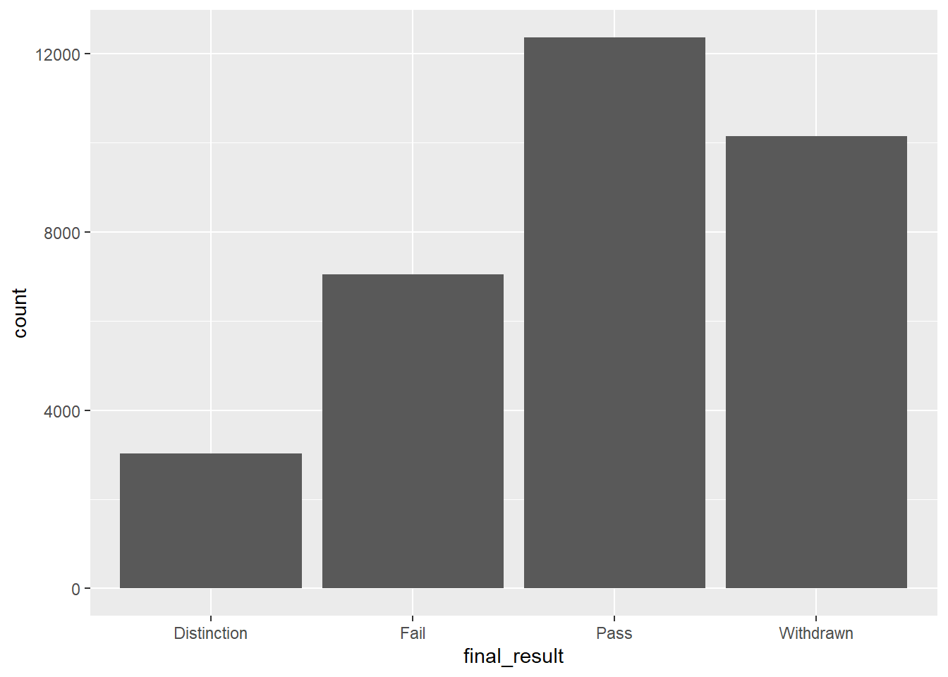
This automatically counts how many students have each final result (Pass, Fail, Distinction, Withdrawn) and displays the counts as bars.
# Stacked bar chart by group
students |>
  ggplot(aes(x = gender, fill = final_result)) +
  geom_bar()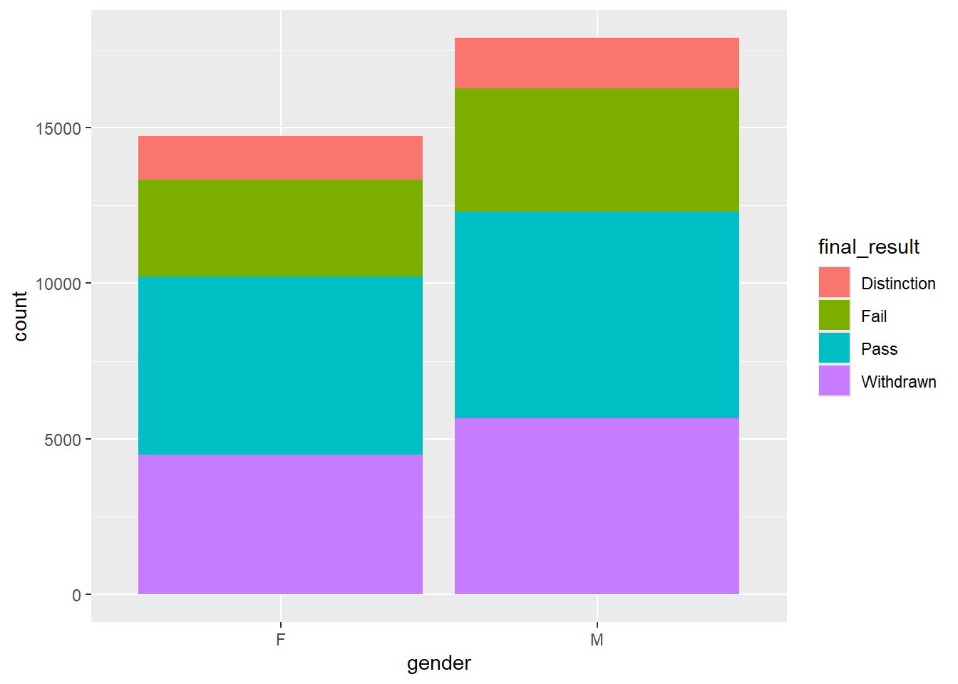
The fill aesthetic colors the bars by final_result, creating stacked bars that show how outcomes differ between genders.
# Side-by-side bars
students |>
  ggplot(aes(x = gender, fill = final_result)) +
  geom_bar(position = "dodge")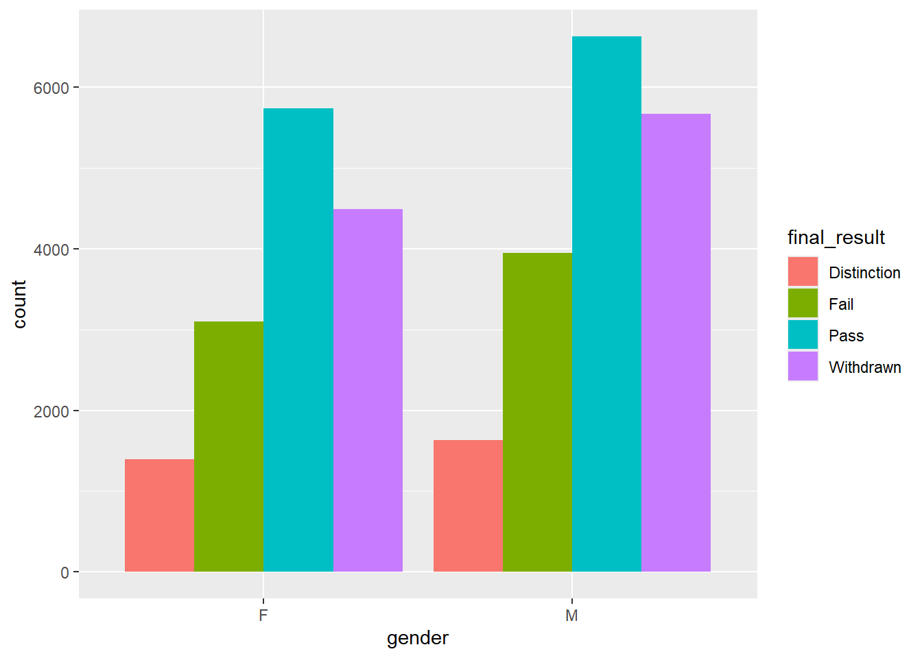
Setting position = "dodge" puts bars next to each other instead of stacking them, making it easier to compare counts directly.
3.7.3 Histograms - Distributions
Use geom_histogram() to see the distribution of continuous variables:
# Distribution of scores
students |>
  ggplot(aes(x = mean_weighted_score)) +
  geom_histogram(binwidth = 50)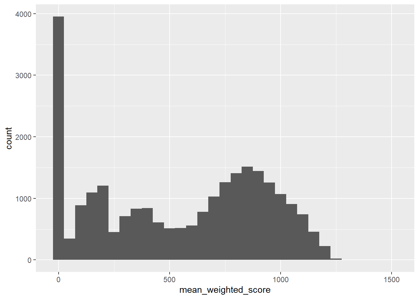
The binwidth argument controls how wide each bar is. Smaller values show more detail, larger values show broader patterns.
# Separate distributions by group
students |>
  filter(!is.na(mean_weighted_score)) |>
  ggplot(aes(x = mean_weighted_score, fill = factor(pass))) +
  geom_histogram(binwidth = 50, position = "identity", alpha = 0.5)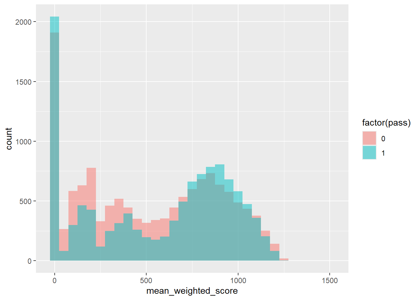
Using position = "identity" overlays the histograms, and alpha = 0.5 makes them semi-transparent so you can see both distributions.
3.7.4 Boxplots - Comparing Distributions
Use geom_boxplot() to compare distributions across groups:
# Scores by final result
students |>
  filter(!is.na(mean_weighted_score)) |>
  ggplot(aes(x = final_result, y = mean_weighted_score)) +
  geom_boxplot()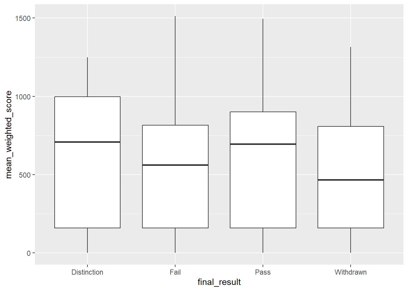
Boxplots show the median (middle line), quartiles (box edges), and outliers (individual points). This makes it easy to see that Distinction students have higher median scores than Pass students, who score higher than those who Fail or Withdraw.
# With colors
students |>
  filter(!is.na(mean_weighted_score)) |>
  ggplot(aes(x = final_result, y = mean_weighted_score, fill = final_result)) +
  geom_boxplot()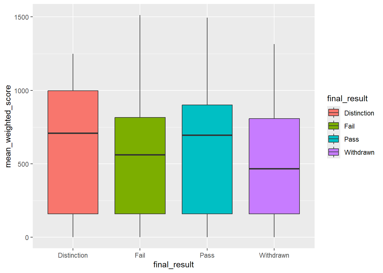
Adding fill colors each boxplot by the category, making them easier to distinguish.
3.7.5 Scatter Plots - Relationships
Use geom_point() to explore relationships between two continuous variables:
# Registration timing vs. scores
students |>
  filter(!is.na(mean_weighted_score)) |>
  ggplot(aes(x = date_registration, y = mean_weighted_score)) +
  geom_point(alpha = 0.3)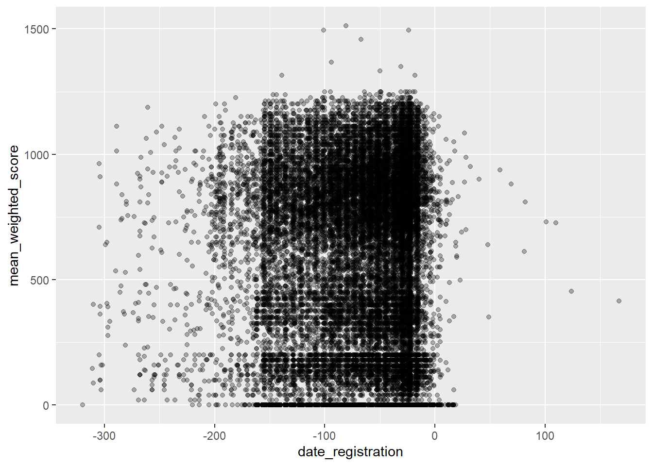
The alpha parameter makes points semi-transparent, which helps when many points overlap. This plot would show whether students who register earlier tend to score higher or lower.
# Add a trend line
students |>
  filter(!is.na(mean_weighted_score)) |>
  ggplot(aes(x = date_registration, y = mean_weighted_score)) +
  geom_point(alpha = 0.3) +
  geom_smooth(method = "lm")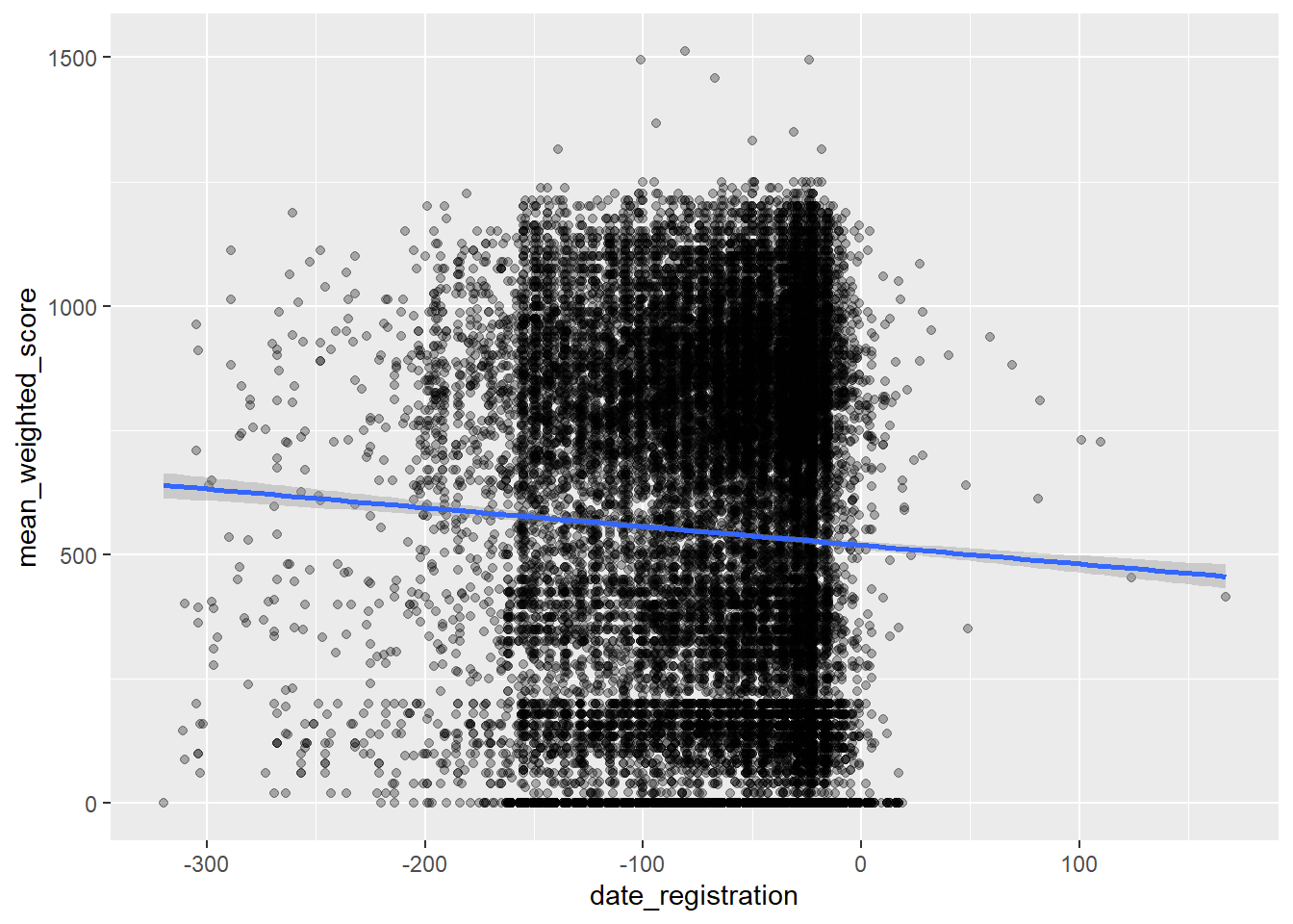
Adding geom_smooth(method = "lm") fits a linear model and displays the trend line with a confidence band, making patterns easier to see.
3.7.6 Improving Plots with Labels and Themes
Good plots need clear labels:
students |>
  ggplot(aes(x = final_result)) +
  geom_bar(fill = "steelblue") +
  labs(
    title = "Distribution of Student Outcomes",
    x = "Final Result",
    y = "Number of Students"
  ) +
  theme_minimal()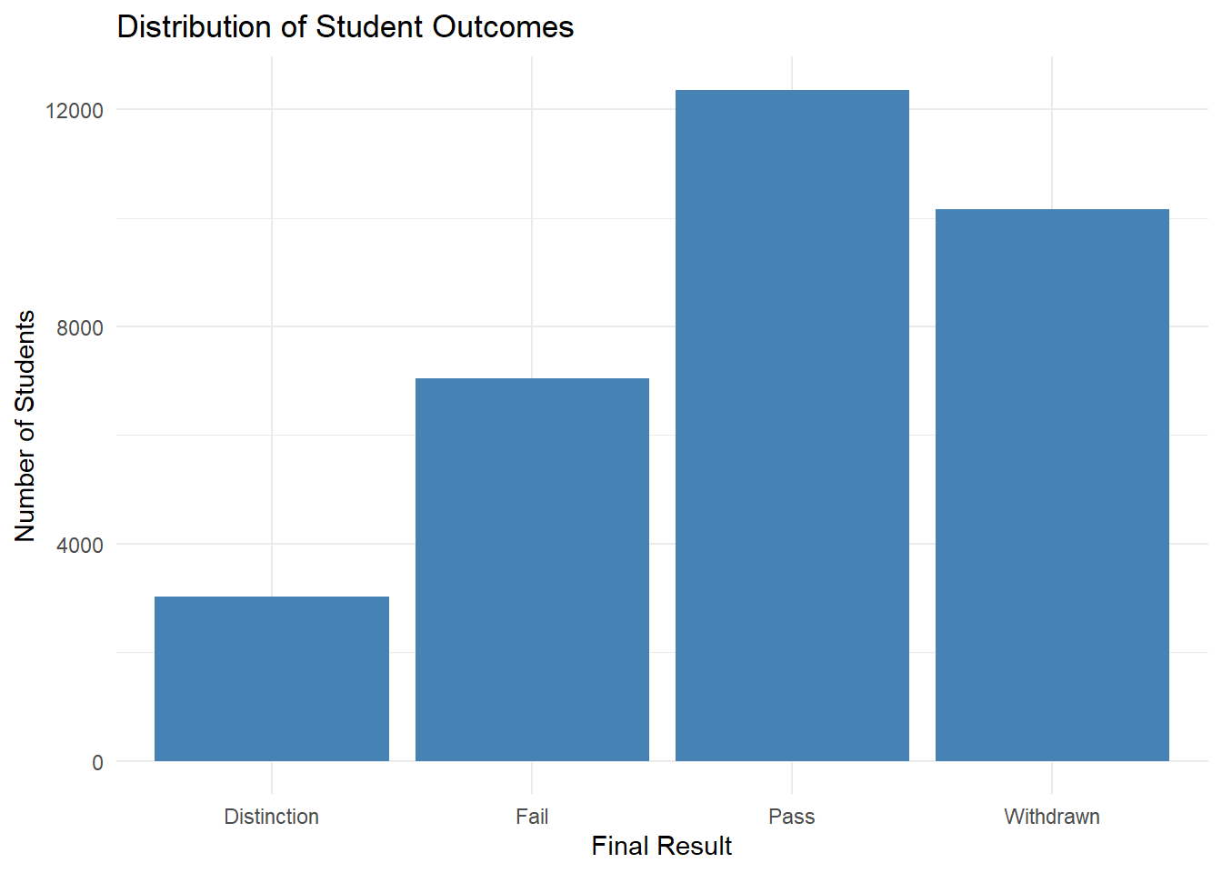
The labs() function adds titles and axis labels. The theme_minimal() function applies a clean, simple theme. Other themes include theme_bw(), theme_classic(), and theme_light().
3.7.7 Faceting - Small Multiples
Use faceting to create separate plots for different groups:
# Separate plot for each course module
students |>
  ggplot(aes(x = final_result)) +
  geom_bar() +
  facet_wrap(~code_module)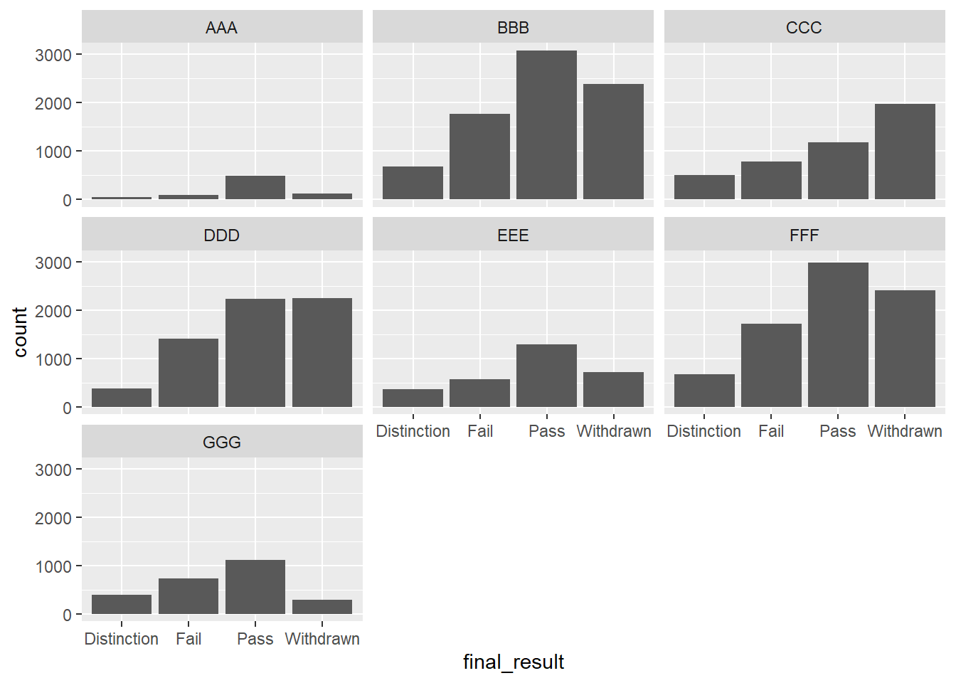
This creates a grid of small bar charts, one for each module. It is useful when you want to compare patterns across many categories.
# Grid by two variables
students |>
  filter(!is.na(mean_weighted_score)) |>
  ggplot(aes(x = mean_weighted_score)) +
  geom_histogram(binwidth = 50) +
  facet_grid(gender ~ disability)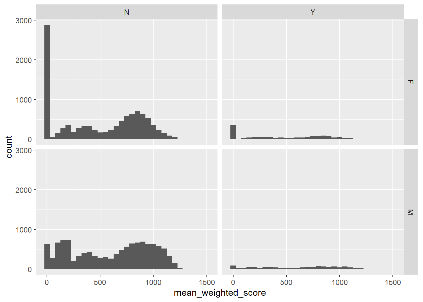
facet_grid() creates a matrix of plots: rows for one variable (gender), columns for another (disability). This lets you see how score distributions vary across combinations of factors.
3.8 Summary
You’ve now seen core tidyverse functions in action with real data. The seven dplyr functions covered here—filter(), select(), mutate(), summarize(), group_by(), arrange(), and count()—handle the majority of everyday data manipulation tasks. The ggplot2 visualizations—bar charts, histograms, boxplots, scatter plots, and faceting—cover most exploratory analysis needs.
The subsequent chapters in this book use these functions extensively, and we will introduce additional tidyverse capabilities as they become relevant. You will continue learning by doing, working with real data and real research questions.
When you want to go deeper:
- R for Data Science (2e): The definitive guide to the tidyverse
- Tidyverse documentation: Reference docs for all packages
- RStudio Cheatsheets: Visual quick references for dplyr, ggplot2, and more
The tidyverse community is large and welcoming. When you get stuck, someone has likely asked your question before.