R

2.1 Overview

We are not going to teach you RStudio comprehensively because excellent resources already exist for that purpose. We particularly recommend R for Data Science, Data Science in Education Using R, the RStudio primers, and Happy Git and GitHub for the useR.

Instead, this chapter covers just enough to reproduce our workflows and extend them to your own data science work. Think of this as the minimal viable setup for doing the work in this book.

2.2 Three Ways to Write R Code

Positron supports multiple file types for writing R code. You will encounter all three in data science work:

2.2.1 R Scripts (.R)

Plain text files containing R code, executed line-by-line or all at once. Great for data processing pipelines, functions, and code you will reuse.

Create one: File → New File → R Script

# This is an R script
# Lines starting with # are comments
data <- read.csv("mydata.csv")
summary(data)

Here is a more realistic example using student assessment data. Save this as explore-data.R:

# Example: Quick data exploration in an R script
library(tidyverse)

# Read the data
students <- read_csv("data/oulad-students-and-assessments.csv")

# Quick summaries
summary(students$mean_weighted_score)
table(students$final_result)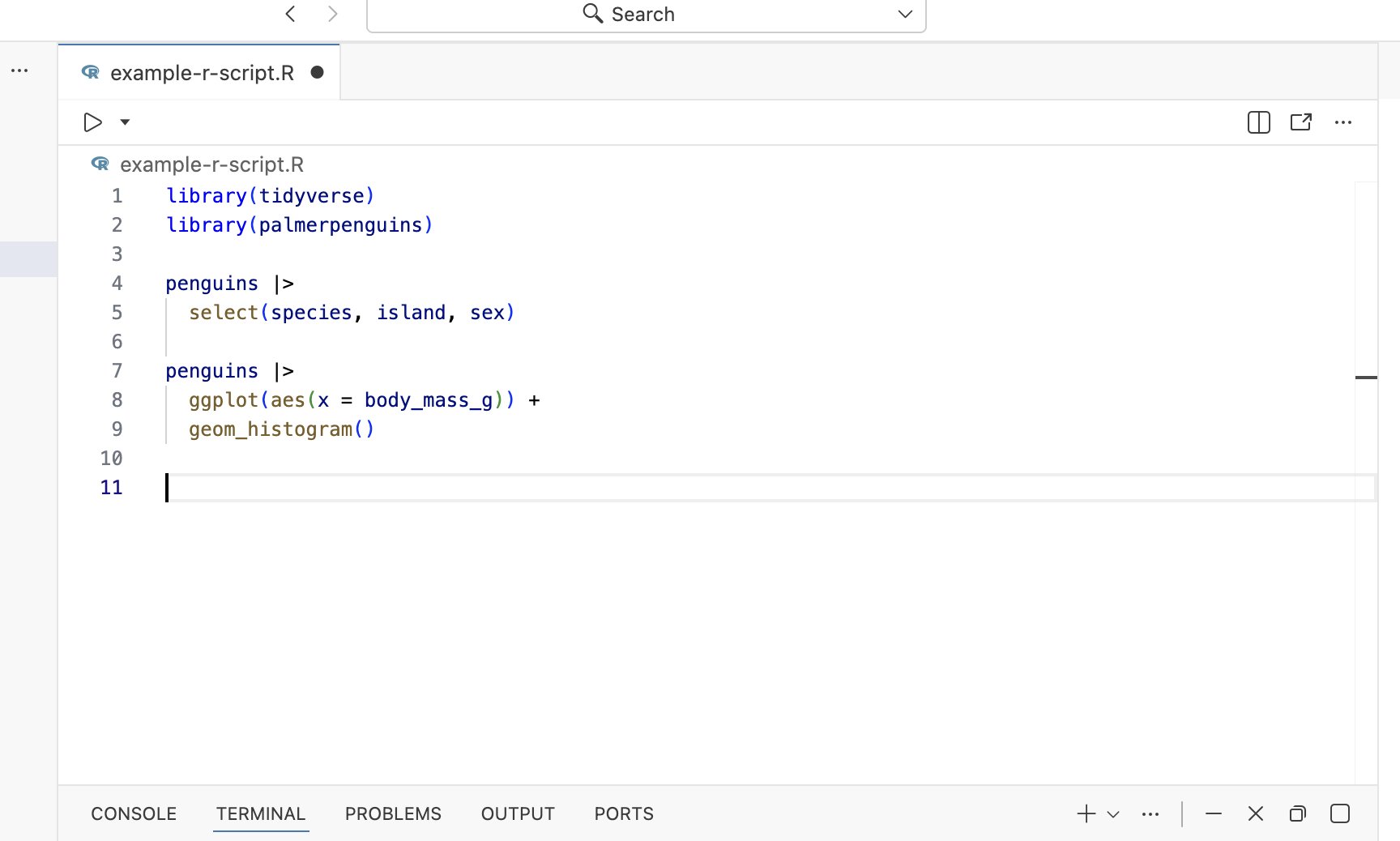

Figure 2.4. R script in the source pane with data-loading and summary commands.

This script loads the tidyverse package (more on this in the next chapter), reads a CSV file, and produces quick summaries. You can run it line-by-line using Cmd/Ctrl + Enter, or run the entire script at once. The output appears in the Console, but the script itself is saved for later use.

2.2.2 R Markdown (.Rmd)

Documents that weave together narrative text (in Markdown) and code chunks. When you “knit” an R Markdown file, it executes the code and generates a formatted document (HTML, PDF, or Word).

You should know R Markdown exists because you will encounter it in older resources and projects, but we are not using it in this book.

2.2.3 Quarto (.qmd)

Quarto is the successor to R Markdown, with better multi-language support (R, Python, Julia) and more consistent syntax. It is what we will use throughout this book.

Create one: File → New File → Quarto Document

The structure looks similar to R Markdown, but the rendering engine is more powerful:

---
title: "My Analysis"
format: html
---

## Introduction

This is regular text.
```{r}
# This is a code chunk
x <- 1:10
mean(x)
```

Click the “Render” button (or Ctrl/Cmd + Shift + K) to execute all code and generate your document.

Here is a more complete Quarto example analyzing student data:

---
title: "OULAD Student Analysis"
format: html
---

## Loading Data

First, we will load the student assessment data from the Open University Learning Analytics Dataset:

```{r}
library(tidyverse)
students <- read_csv("data/oulad-students-and-assessments.csv")
```

## Pass Rates by Gender

Let us examine how pass rates differ by gender:

```{r}
students |>
  group_by(gender, pass) |>
  count() |>
  pivot_wider(names_from = pass, values_from = n)
```

The table above shows the number of students who passed (1) and did not pass (0) for each gender. We can see that both groups have substantial representation in the dataset.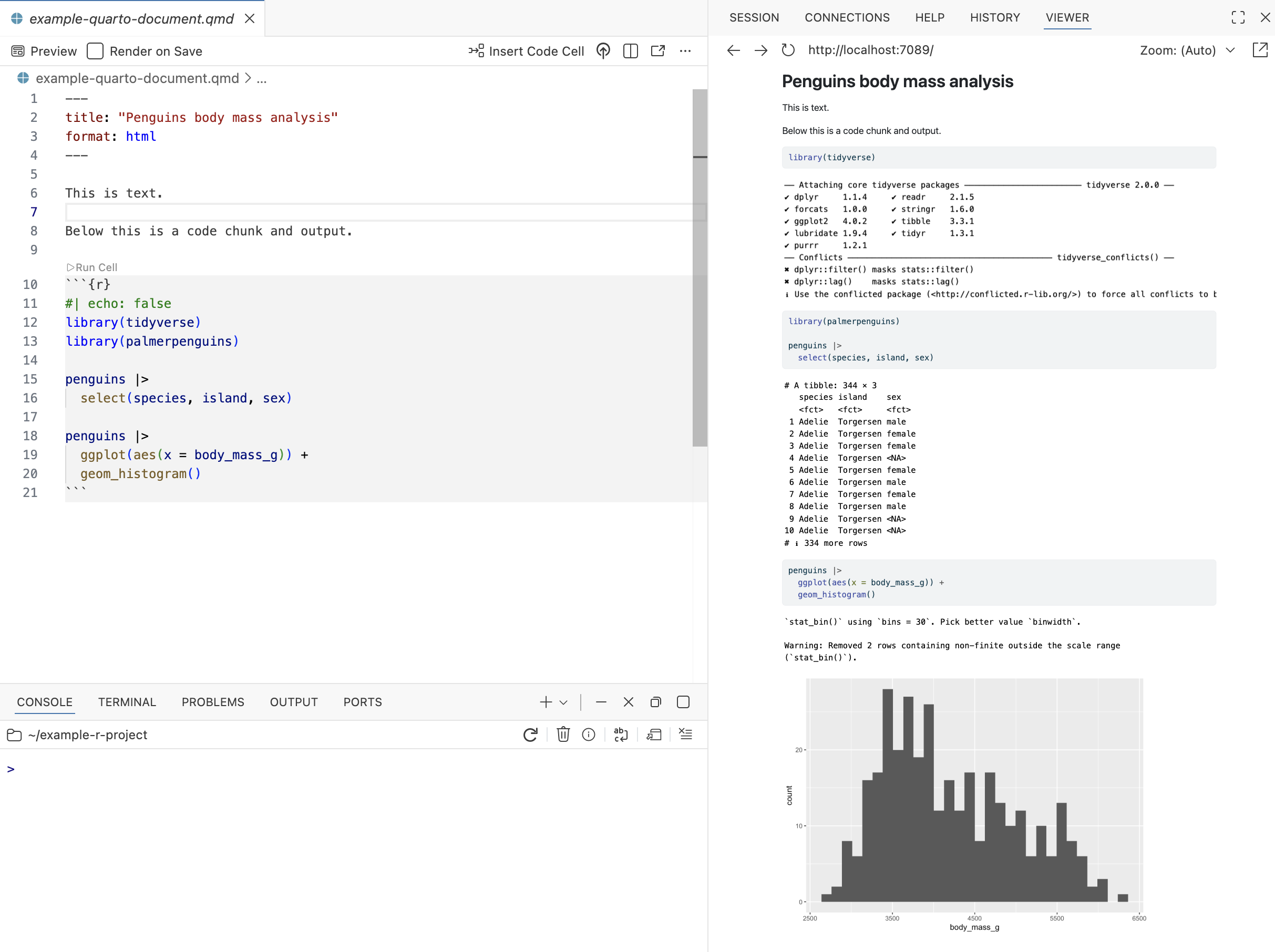

Figure 2.5. Rendered Quarto document combining narrative, code, and output.

When you render this document, Quarto executes each code chunk in order, captures the output, and weaves it together with your explanatory text. The result is an HTML document where readers see your code, your results, and your interpretation all together. This makes your analysis reproducible in that anyone with your data can re-run your Quarto file and get the same results.

Key difference for beginners: Think of R scripts as “just code” and Quarto as “code + explanation + output” in one document. Use scripts for behind-the-scenes work, Quarto for analysis you want to share or understand later.

2.2.4 Controlling Chunk Behavior with Options

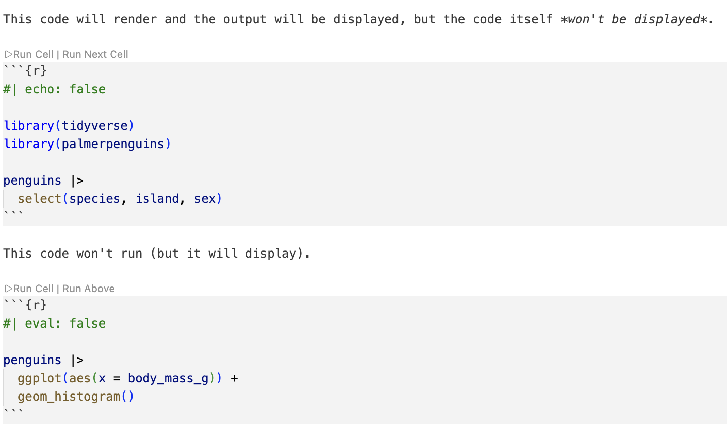
Quarto lets you control what appears in your rendered document using chunk options. These are specified at the top of each code chunk using #| syntax.

Common options include:

#| echo: false — Hide the code, show only the output
#| eval: false — Show the code but do not run it
#| warning: false — Suppress warning messages
#| message: false — Suppress messages (like package loading notifications)
#| fig-width: 8 and #| fig-height: 6 — Control plot dimensions in inches

Here is an example showing how to hide code while displaying a plot:

```{r}
#| echo: false
#| message: false

library(tidyverse)
students <- read_csv("data/oulad-students-and-assessments.csv")

students |>
  ggplot(aes(x = final_result)) +
  geom_bar() +
  labs(title = "Distribution of Final Results")
```

Figure 2.6. Quarto chunk options for controlling code visibility and execution output.

When rendered, readers see the plot but not the code that created it. This is useful for final reports where you want to emphasize results rather than implementation details.

You can also set options globally for the entire document by adding them to your YAML header. For example, to hide all code by default:

---
title: "My Analysis"
format: html
execute:
  echo: false
---

Individual chunks can override global settings. For more options, see the Quarto documentation on execution options.

2.3 Console vs. Source: Exploration vs. Preservation

A common pattern in data science work:

Console: Quick exploration, testing ideas, checking output. Code here disappears when you close Positron.
Source (scripts/Quarto): Code you want to keep, reproduce, or share. This is your permanent record.

Here is what this looks like in practice. Try this in the Console for a quick calculation:

# In Console - just exploring
mean(c(85, 92, 78, 95, 88))
[1] 87.6

That is useful for a quick check, but if you want to preserve this process for later:

# In a script - keeping a record
test_scores <- c(85, 92, 78, 95, 88)
average_score <- mean(test_scores)
print(average_score)

The second approach creates a record you can return to, modify, and share. If you later need to change the scores or calculate something else, the script preserves your workflow.

Early on, you might type everything in the Console. That is fine for learning! But as soon as you do something you want to remember, put it in a script or Quarto file.

2.4 When You Get Stuck

2.4.1 Reading Error Messages

When something goes wrong, R prints an error message in the Console (usually in red). These messages often look cryptic at first, but they are trying to help:

Error in mean(x) : object 'x' not found

This tells you exactly what went wrong: R could not find an object called x. Either you misspelled it, or you have not created it yet.

2.4.2 Getting Help on Functions

R has built-in documentation for every function:

?mean           # Opens help for the mean() function
??regression    # Searches all help files for "regression"

Help files include descriptions, arguments, examples, and related functions.

2.5 Summary

This chapter covered the essential R skills needed to follow the workflows in this book: writing code in scripts, R Markdown, and Quarto documents; loading and inspecting data; computing basic summaries; producing simple visualizations; and reading error messages when things go wrong. These fundamentals carry through every subsequent chapter.

2.5.1 Large Language Models and AI Tools for Getting Unstuck

In Section 3, we cover using large language models as part of a research workflow. But LLMs are also useful for getting unstuck when you are learning and this is increasingly how working data scientists operate.

Two approaches work well:

Ask LLMs directly: ChatGPT, Claude, or your preferred model can explain error messages, suggest debugging approaches, and clarify confusing documentation. Copy your error message, describe what you were trying to do, and ask for help.
Use AI tools directly in Positron: AI coding assistants can work inside your editor to suggest code completions, explain what existing code does, and generate boilerplate. We will cover how to set these up in the next section.

The best programmers do not memorize every function—they know how to find answers quickly. LLMs have become part of that toolkit, alongside documentation, Stack Overflow, and experimentation. Use them when you are stuck, but also pay attention to why solutions work. That is how you build intuition.

2.5.1.1 Using AI Tools Directly in Positron

Positron, being built on VS Code, supports AI assistant extensions that can help you write code more efficiently and understand errors more quickly.

Positron Assistant

Positron includes a built-in AI chat panel called Positron Assistant. You can open it from the sidebar (look for the chat icon) or with the keyboard shortcut Ctrl/Cmd + Shift + I. Positron Assistant is context-aware—it can see your open files, your console history, and the variables in your environment, so you can ask questions about your code without copying and pasting everything into an external tool.

For example, if you have just loaded a dataset and are not sure how to reshape it, you can highlight the relevant code and ask the assistant to explain it, suggest next steps, or help you fix an error. You can also ask it to generate code from a plain-language description, like “make a bar chart of pass rates by gender.” The assistant will write code that fits the context of your current session, using the packages you have already loaded and the data you are working with.

Positron Assistant connects to a language model provider that you configure in your settings—options include Anthropic (Claude), OpenAI, and others. Some providers require a paid API key; check Positron’s documentation at https://positron.posit.co/ for current setup instructions. Because the assistant runs inside Positron rather than in a separate browser tab, it reduces the friction of switching between your code and a help tool, which makes it especially useful when you are learning.

When to Use Inline AI vs. External LLMs

Different tools excel at different tasks:

Inline AI (Copilot): Quick code completions, writing repetitive code, remembering function syntax, generating common patterns
External LLMs (ChatGPT/Claude): Complex explanations, understanding concepts, debugging logic errors, learning new approaches

Many programmers use both: Copilot for day-to-day coding, external LLMs when they are truly stuck or learning something new.

Important Caution

AI suggestions are not always correct. Always review code before accepting it, especially for data analysis where subtle errors can lead to wrong conclusions. Use AI tools to speed up your work, but verify that the code does what you think it does.

Please see LLM Methods section (intro) for more information about the relationship between you, data, and LLMs.