Create latent profile plots

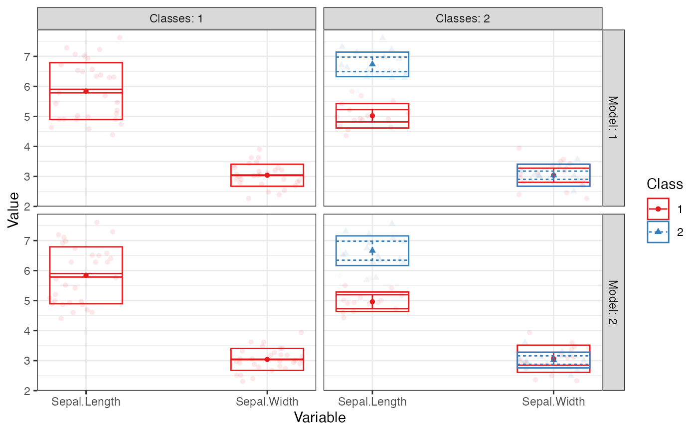
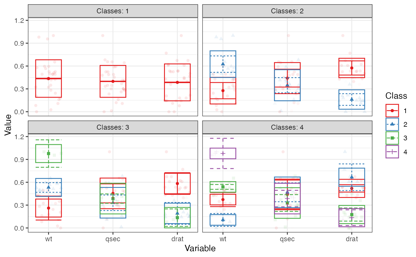
Creates a profile plot according to best practices, focusing on the visualization of classification uncertainty by showing:

1. Bars reflecting a confidence interval for the class centroids

2. Boxes reflecting the standard deviations within each class; a box encompasses +/- 64% of the observations in a normal distribution

3. Raw data, whose transparancy is weighted by the posterior class probability, such that each datapoint is most clearly visible for the class it is most likely to be a member of.

plot_profiles(
  x,
  variables = NULL,
  ci = 0.95,
  sd = TRUE,
  add_line = TRUE,
  rawdata = TRUE,
  bw = FALSE,
  alpha_range = c(0, 0.1),
  ...
)

# S3 method for default
plot_profiles(
  x,
  variables = NULL,
  ci = 0.95,
  sd = TRUE,
  add_line = FALSE,
  rawdata = TRUE,
  bw = FALSE,
  alpha_range = c(0, 0.1),
  ...
)

Arguments

x	An object containing the results of a mixture model analysis.
variables	A character vectors with the names of the variables to be plotted (optional).
ci	Numeric. What confidence interval should the errorbars span? Defaults to a 95% confidence interval. Set to NULL to remove errorbars.
sd	Logical. Whether to display a box encompassing +/- 1SD Defaults to TRUE.
add_line	Logical. Whether to display a line, connecting cluster centroids belonging to the same latent class. Defaults to TRUE. Note that the additional information conveyed by such a line is limited.
rawdata	Should raw data be plotted in the background? Setting this to TRUE might result in long plotting times.
bw	Logical. Should the plot be black and white (for print), or color?
alpha_range	The minimum and maximum values of alpha (transparancy) for the raw data. Minimum should be 0; lower maximum values of alpha can help reduce overplotting.
...	Arguments passed to and from other functions.

Value

An object of class 'ggplot'.

Author

Caspar J. van Lissa

Examples

# Example 1
iris_sample <- iris[c(1:10, 51:60, 101:110), ] # to make example run more quickly

iris_sample %>%
 subset(select = c("Sepal.Length", "Sepal.Width")) %>%
 estimate_profiles(n_profiles = 1:2, models = 1:2) %>%
 plot_profiles()
#> The 'variances'/'covariances' arguments were ignored in favor of the 'models' argument.

# Example 2

# \donttest{
mtcars %>%
  subset(select = c("wt", "qsec", "drat")) %>%
  poms() %>%
  estimate_profiles(1:4) %>%
  plot_profiles(add_line = F)
# }